CircTest module
The CircTest module of circtools allows to test the variation of circRNAs in respect to host genes. It is recommended to work with the output of the circtools detect module, but can also run on custom count tables. Required are one table with circular RNA counts and one table containing with host-gene counts. These tables have to have the same order, i.e. circ[i,j] and linear[i,j] are read-counts for the same circRNA in the same sample.
The circtools circtest module is based on the equally named R package CircTest
Required tools and packages
circtools circtest depends on R and the following R packages:
- aod
- ggplot2
- plyr
The CircTest R package as well as all dependencies are installed during the circtools installation procedure.
Manual installation instructions
The following commands have to be performed within an R shell:
> install.packages("devtools")
> require(devtools)
> install_github('dieterich-lab/CircTest')
> library(CircTest)
Usage with circtools detect data
A call to circtools circtest --help shows all available command line flags:
usage: circtools [-h] -d DCC_DIR -l CONDITION_LIST -c CONDITION_COLUMNS -g
                 GROUPING [-r NUM_REPLICATES] [-f MAX_FDR] [-p PERCENTAGE]
                 [-s FILTER_SAMPLE] [-C FILTER_COUNT] [-o OUTPUT_DIRECTORY]
                 [-n OUTPUT_NAME] [-m MAX_PLOTS] [-a LABEL] [-L RANGE]
                 [-O ONLY_NEGATIVE] [-H ADD_HEADER] [-M {colour,bw}]

circular RNA statistical testing - Interface to https://github.com/dieterich-lab/CircTest

optional arguments:
  -h, --help            show this help message and exit

Required:
  -d DCC_DIR, --DCC DCC_DIR
                        Path to the detect/DCC data directory
  -l CONDITION_LIST, --condition-list CONDITION_LIST
                        Comma-separated list of conditions which should be
                        comparedE.g. "RNaseR +","RNaseR -"
  -c CONDITION_COLUMNS, --condition-columns CONDITION_COLUMNS
                        Comma-separated list of 1-based column numbers in the
                        detect/DCC output which should be compared; e.g.
                        10,11,12,13,14,15
  -g GROUPING, --grouping GROUPING
                        Comma-separated list describing the relation of the
                        columns specified via -c to the sample names specified
                        via -l; e.g. -g 1,2 and -r 3 would assign sample1 to
                        each even column and sample 2 to each odd column

Processing options:
  -r NUM_REPLICATES, --replicates NUM_REPLICATES
                        Number of replicates used for the circRNA experiment
                        [Default: 3]
  -f MAX_FDR, --max-fdr MAX_FDR
                        Cut-off value for the FDR [Default: 0.05]
  -p PERCENTAGE, --percentage PERCENTAGE
                        The minimum percentage of circRNAs account for the
                        total transcripts in at least one group. [Default:
                        0.01]
  -s FILTER_SAMPLE, --filter-sample FILTER_SAMPLE
                        Number of samples that need to contain the amount of
                        reads specified via -C [Default: 3]
  -C FILTER_COUNT, --filter-count FILTER_COUNT
                        Number of CircRNA reads that each sample specified via
                        -s has to contain [Default: 5]

Output options:
  -o OUTPUT_DIRECTORY, --output-directory OUTPUT_DIRECTORY
                        The output directory for files created by circtest
                        [Default: .]
  -n OUTPUT_NAME, --output-name OUTPUT_NAME
                        The output name for files created by circtest
                        [Default: circtest]
  -m MAX_PLOTS, --max-plots MAX_PLOTS
                        How many of candidates should be plotted as bar chart?
                        [Default: 50]
  -a LABEL, --label LABEL
                        How should the samples be labeled? [Default: Sample]
  -L RANGE, --limit RANGE
                        How should the samples be labeled? [Default: Sample]
  -O ONLY_NEGATIVE, --only-negative-direction ONLY_NEGATIVE
                        Only print entries with negative direction indicator
                        [Default: False]
  -H ADD_HEADER, --add-header ADD_HEADER
                        Add header to CSV output [Default: False]
  -M {colour,bw}, --colour {colour,bw}
                        Can be set to bw to create grayscale graphs for
                        manuscripts
Sample call
As for the other module tutorials, we use the Jakobi et al. 2016 data set from the detection module in this module. Below is the sample call for the newly generated circtools detect data:
circtools circtest -d 01_detect/ -p 0.01 -s 3 -r 4 -C 2 -g 1,2,1,2,1,2,1,2 -l RNaseR-,RNaseR+ -c 4,5,6,7,8,9,10,11 -o 04_circtest/
Here we have the DCC data located in the folder 01_detect/, the experiment had 2 conditions, listed via -l RNaseR-,RNaseR+, the samples in the circtools detect data file are sorted in the the order specified via -g 1,2,1,2,1,2,1,2, i.e. there are 4 RNaseR- samples and 4 RNaseR+ samples. These 4+4=8 columns are found in the circtools detect data file in the columns specified via -c 4,5,6,7,8,9,10,11.
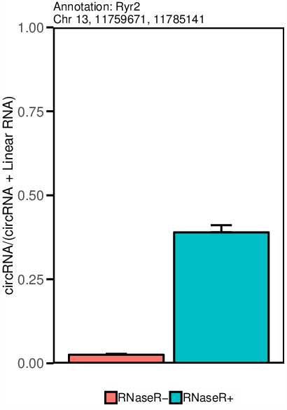
Output files
The circtest module creates an .xlsx file that contains all circRNA candidates passing the statistical test with the given values, as well as the raw data files. Additionally a .pdf file is generated that contains a graphical representation of the top significant circRNAs (see sample picture).
Usage with external count data
Additional to the built-in functionality to use directly use the data files produced by circtools detect it is also possible to use generic count tables. In this case however, the underlying R package CircTest has to be used directly. The input tables may have many columns describing the circle or just one column containing the circle ID followed by many columns of read counts.
Example count table for back-spliced reads (Circular.csv)
| CircID | Control_1 | Control_2 | Control_3 | Treatment_1 | Treatment_2 | Treatment_3 |
|---|---|---|---|---|---|---|
| chr1:100|800 | 0 | 2 | 1 | 5 | 4 | 0 |
| chr1:1050|10080 | 20 | 22 | 21 | 10 | 13 | 0 |
| chr2: 600|1000 | 0 | 1 | 0 | 10 | 0 | 1 |
| chr10:4100|5400 | 55 | 54 | 52 | 56 | 53 | 50 |
| chr11:600|1500 | 3 | 0 | 1 | 2 | 2 | 3 |
Example table for host-gene reads (Linear.csv)
| CircID | Control_1 | Control_2 | Control_3 | Treatment_1 | Treatment_2 | Treatment_3 |
|---|---|---|---|---|---|---|
| chr1:100|800 | 10 | 11 | 12 | 9 | 10 | 10 |
| chr1:1050|10080 | 80 | 281 | 83 | 45 | 48 | 46 |
| chr2: 600|1000 | 5 | 5 | 2 | 12 | 8 | 7 |
| chr10:4100|5400 | 101 | 110 | 106 | 150 | 160 | 153 |
| chr11:600|1500 | 20 | 21 | 18 | 19 | 20 | 20 |
Sample R calls to work with generic data
- Read in tables
Circ <- read.delim('Circ.csv', header = T, as.is = T)
Linear <- read.delim('Linear.csv', header = T, as.is = T)
- Filter tables
To model expression data using the beta binomial distribution and testing for differences in groups, it is beneficial to only test well supported circles. Users may use the package’s function Circ.filter() to filter the input data. The function has the following parameters:
Nreplicates: specifies the number of replicates in each conditionfilter.sample: specifies the number of samples the circle has to have enough circular reads in to be considered.filter.count: specifies the circular read count threshold.percentage: specifies the minimum circle to host-gene ratio.circle_description: tells the function which columns are NOT filled with read counts but the circle’s annotation.
# filter circles by read counts
Circ_filtered <- Circ.filter(circ = Circ, linear = Linear, Nreplicates = 3, filter.sample = 3, filter.count = 5, percentage = 0.1, circle_description = 1)

#            CircID Control_1 Control_2 Control_3 Treatment_1 Treatment_2 Treatment_3
# 2 chr1:1050|10080        20        22        21          10          13           0
# 4 chr10:4100|5400        55        54        52          56          53          50


# filter linear table by remaining circles
Linear_filtered <- Linear[rownames(Circ_filtered),]

#            CircID Control_1 Control_2 Control_3 Treatment_1 Treatment_2 Treatment_3
# 2 chr1:1050|10080        80        81        83          45          48          46
# 4 chr10:4100|5400       101       110       106         150         160         153
- Test for changes
Circ.test uses the beta binomial distribution to model the data and performs an ANOVA to identify circles which differ in their relative expression between the groups. It is important that the grouping is correct (group) and the non-read-count columuns are specified (circle_description).
test <- Circ.test(Circ_filtered, Linear_filtered, group=c(rep(1,3),rep(2,3)), circle_description = 1)
$summary_table
           CircID      sig_p
4 chr10:4100|5400 0.01747407

# $sig.dat
#            CircID Control_1 Control_2 Control_3 Treatment_1 Treatment_2 Treatment_3
# 4 chr10:4100|5400        55        54        52          56          53          50

$p.val
[1] 0.153464107 0.008737037

$p.adj
[1] 0.15346411 0.01747407

$sig_p
[1] 0.01747407
- Visualize data
The CircTest library features a built-in plotting functions to view significantly different genes. Sample code for visualizing the ratio as barplot might be something like:
for (i in rownames(test$summary_table))  {
  Circ.ratioplot(Circ_filtered, Linear_filtered, plotrow=i, groupindicator1=c(rep('Control',3),rep('Treatment',3)),
                 lab_legend='Condition', circle_description = 1 )
}
In order to visualize the abundance of host-gene and circle separately in a line plot try
 for (i in rownames(test$summary_table))  {
   Circ.lineplot(Circ_filtered, Linear_filtered, plotrow=i, groupindicator1=c(rep('Control',3),rep('Treatment',3)),
                 circle_description = 1 )
}